The James-Stein Estimator

This write up is about an estimator. A statistical estimator, is used when you already have a model in mind, data at hand and want to estimate some parameters needed for the model. For example, you want to predict how many runs a batter would make in a game given recent history \(x_1,x_2,x_3,\ldots\) . If we assume (we are making a choice of a model now) that the scores come from a normal distribution with mean \(\mu\) and standard deviation \(\sigma\) then the probability density function for a given value \(x\) is

The likelihood that a series of points \(x_1,x_2,x_3,\ldots\) come from such a distribution can be expressed as

Next is basic calculus. Take the logarithm on both sides, set the partial derivative w.r.t. \(\mu\) to zero yields (excluding the algebra)

To verify, you also need to check the second derivative's sign to see if its negative to ensure that it is indeed a maxima you have found.

So a simple estimator would be to use the average runs scored from the past \(n\) days. The average is the result of a "maximum likelihood" approach briefly described above.What if you had 5 players you wanted to estimate the average for? Intuition would tell you that you should simply compute the average for each. Wrong! The James-Stein approach provides a way to pool the data such that the overall error made in estimation is minimized.

Specifically, I'll demonstrate the James-Stein estimator. It is a surprising result discovered by Charles Stein and later formalized by Willard James on estimating such parameters. What makes it stunning is the rather counter intuitive result it demonstrates. James-Stein's estimator approach states that if you wanted to simultaneously estimate a set of independent parameters from data, the maximum likelihood approach is only optimal if you have lesser than 3 parameters to estimate from! If you have more than 3, you are better off using the James-Stein estimator. There is an obvious thought experiment you can think of. If you really wanted just one parameter, could you not simply add an unrelated set of numbers, improve efficiency in estimation and then just use the parameter you are interested in? That's a flaw. The estimator works by minimizing the overall error in estimation so it may make more errors in some of the variables, lesser on others. But overall it will be better than just doing an individual maximum likelihood estimate on each variable. So you could use it if you don't mind seeing slightly bigger errors on some variables, smaller on others but lower overall error.

To see this work, I'll step through the actual algorithm in R. For more details you can refer the wikipedia entry here.The general approach is the following.

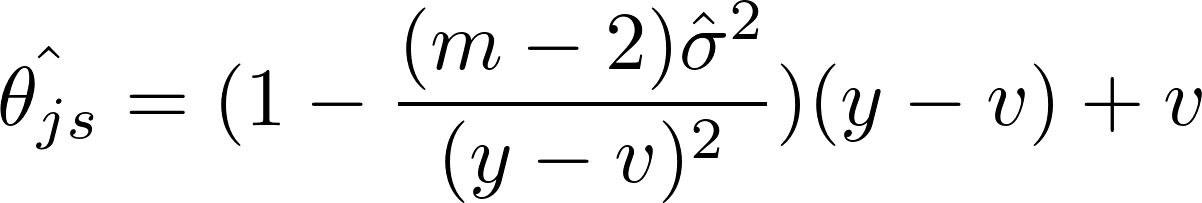
Let

• \(\hat\theta_{js}\) is the James-Stein estimate of the parameters we are interested in computing.
• \(y\) be the set of values observed.
• \(\hat{\sigma}^{2}\) be the estimated variance for all parameters
• \(v\) be the mean of all parameters

then the James Stein estimator is given by

#!/usr/bin/Rscript
 
suppressMessages(library(data.table))
suppressMessages(library(ggplot2))
 
# n.rows is the number of samples we have
n.rows = 100
 
# n.params is the number of parameters
# we want to estimate
n.params = 30
 
# wins will hold the number of times
# the JS estimator beats the MLE estimate
wins   = c()
msejs  = c()
msemle = c()
 
for(iter in seq(1:1000)){
    # Create a sample of parameters
    # They have a range of 20-25
    x.act  = sample(20:25,size=n.params,replace=TRUE)
 
    # Now create a normal distribution for each of the parameters
    # uncomment below if you want to test it for a poisson distribution
    # m = mapply(rpois,mean=x.act,MoreArgs=list(n = n.rows))
    m = mapply(rnorm,mean=x.act,MoreArgs=list(n = n.rows,sd=10))
 
    # Find the global mean
    mbar = mean(colMeans(m))
 
    # Find the column means
    mu0   = colMeans(m)
 
    # Find global variance
    s2 = var(as.vector(m))/(n.rows*n.params)
 
    # Compute the adjustment value
    cval    = 1 - ((n.params - 2)*s2/sum((mu0 - mbar)^2))
 
    # Compute the JS estimate for your parameters
    jsest = mbar + cval *(mu0 - mbar)
    z = data.table(
        actual = x.act,
        mle.est = mu0,
        js.est = jsest)
 
    # Check to see if the JS estimate is better than MLE
    z[,counter := ifelse(abs(js.est - actual) < abs(mle.est - actual),1,0)]
 
    # In case you want to see what the numbers are for the
    # difference between absolute and actual estimates for
    # JS and MLE
    z[,jserr  := abs(js.est - actual)]
    z[,mleerr := abs(mle.est - actual)]
 
    # Record the wins for this iteration of the simulation
    # Repeat.
    wins[iter]   = sum(z$counter)
    msejs[iter]  = sum(z$jserr)
    msemle[iter] = sum(z$mleerr) 
}
 
# What are the mean wins? 
mean(wins)
 
# What are the distribution of the mean wins
quantile(wins,prob = seq(0.1,0.9,by=0.1))
 
z = data.frame(wins = wins)
p = ggplot(z,aes(wins)) +
    geom_histogram(fill='light blue') +
    theme_bw() +
    ggtitle('Of the 30 parameters we wish to estimate:\n how many of them have estimates closer to the actual using the James-Stein estimator than the MLE?') +
    ylab('') +
    xlab('') +
    geom_vline(aes(xintercept=mean(wins),linetype='longdash',colour='blue')) +
    annotate('text',x=18,y=150,label='Mean -->') +
    theme(legend.position='none')
 
png('xyz.png',width=800,height=500)
print(p)
dev.off()

The above R code runs a simulation of sorts. It starts by making some random parameters you would want to estimate and simulates some normally distributed data from it. Next, it uses the James Stein estimator and estimates the very parameters it started off with, using the data. Finally, it compares and records how often the James Stein estimator was better/closer that the MLE estimate. The results from the simulation are shown below.

For kicks, you can try it for a Poisson distribution too, here is what the distribution looks like.

If you are interested in learning more about probability here are a list of books that are good to buy.