Linear Regression, Transforms and Regularization

Follow @ProbabilityPuz

This write up is about the simple linear regression and ways to make it robust to outliers and non linearity. The linear regression method is a simple and powerful method. It is powerful because it helps compress a lot of information through a simple straight line. The complexity of the problem is vastly simplified. However being so simple comes with its set of limitations. For example, the method assumes that after a fit is made, the differences between the predicted and actual values are normally distributed. In reality, we rarely run into such ideal conditions. Almost always there is non-normality and outliers in the data that makes fitting a straight line insufficient. However there are some tricks you could do to make it better.

Statistics: A good book to learn statistics

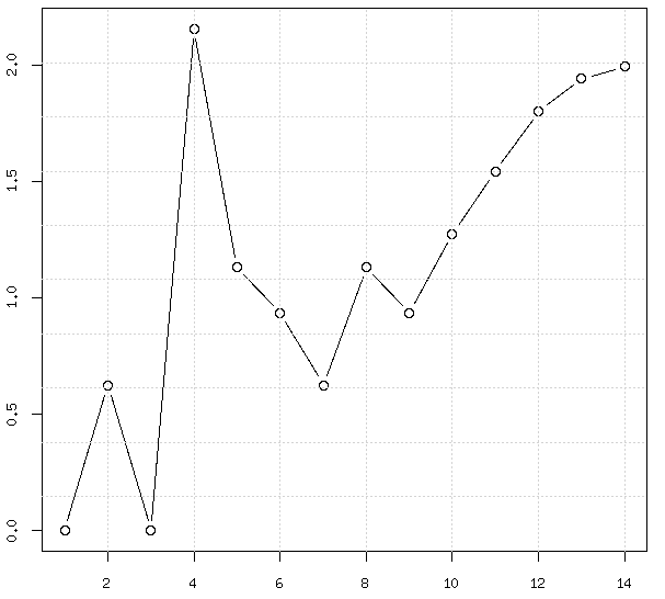
As an example data set consider some dummy data shown in the table/chart below. Notice, value 33 is an outlier. When charted. you can see there is some non-linearity in the data too, for higher values of \(x\)

First lets tackle the non-linearity. The non-linearity can be managed by doing a transformation onthe y-values using the box-cox transform which is a class of power transformation. It is a useful transform to bring about normality in time series values that looks "curvy". The transform looks like
$$
\hat{y} = \frac{y^{\lambda} - 1}{\lambda}
$$
The value of lambda needs to be chosen optimally that maximizes the log likelihood that would make the time series more like it came from a normal distribution. Most statistical tools out there do it for you. In R, the function "boxcox" in the package "MASS" does it for you. The following code snippet computes the optimal value of \(\lambda\) as -0.30303

Let's apply this transformation to the data and see how it looks on a chart.

You can see that it looks a lot better and more like a straight line, except for the outlier at \(x = 4\). The goodness of straight line fit is measured by the fit's \(R^2\) value. The \(R^2\) value tries to quantify the amount of variance that can be explained by the fit. If we fitted a straight line through the original data we get an \(R^2 = 0.06804 \), and the transformed data yields an \(R^2 = 0.4636\) demonstrating an improvement. Next, lets try and manage the outlier. If you try fitting a straight line \(y = \alpha_0 + \alpha_{1} x\) through a set of points that have a few outliers you will notice that the values of \(\alpha_{0}, \alpha_{1}\) tend to be slightly large. They end up being slightly large because the fit is trying to "reach out" and accommodate the outlier. In order to minimize the effect of the outlier we get back into the guts of the linear regression. A linear regression typically tries to minimize the overall error \(e\) as computed as
$$
e = \sum_{i=1}^{N}\frac{(y_{actual} - \alpha_{0} - \alpha_{1}x)^2}{N}
$$
where \(N\) is the number of points. We can tweak the above equation to minimize as follows
$$
e = \sum_{i=1}^{N}\frac{(y_{actual} - \alpha_{0} - \alpha_{1}x)^2}{N} + \lambda(\alpha_{0}^2 + \alpha_{1}^2)
$$
The tweaked error equation forces towards choices of \(\alpha_{0}, \alpha_{1}\) where they cannot take larger values. The optimal value of \(\lambda\) needs to be ascertained by tuning. A formulaic solution does not exist, so we use another tool in R, the function "optim". This function lets you do basic optimization and minimizes any function you pass it, along with required parameters. It returns parameter values that minimize this function. The actual usage of this function isn't exactly intuitive. Most examples on the internet talk of minimizing a proper well formed function. Most real life applications involve minimizing functions having lots of parameters and additional data. The funct"optim" accepts the "..." argument which is a means to pass through arguments to the function you want to minimize. So here is how you would do it in R, all of it.

The above code walks through this example by calling optim. It finally outputs the fits in original domain using all three methods

1. The grey line represents the fit if you simply used "lm"
2. The red line represents the fit if you transformed the data and used "lm" in the transformed domain but without regularization. Note: you are clearly worse off.
3. The blue dotted line shows the fit if you used transformation and regularization, clearly a much better fit

The function "optim" has lots of methods that it uses for finding the minimum value of the function. Typically, you may also want to poke around with the best value of \(\lambda\) in the minimization function to get better fits.
If you are looking to buy some books on time series analysis here is a good collection. Some good books to own for probability theory are referenced here